Linear Regression : Implementation using Normal Equation

Normal Equation: Intuition

Normal Equations is a method to solve for $\theta$ analytically.

The first step is to convert or represent the dataset in a Matrix and vector form.

Consider the dataset:

The variables here are the predictors ($x_1,x_2,x_3,x_4$) and the outcome $y$. The coefficients will be $\theta_0,\theta_1, \theta_2, \theta_3 and \theta_4$.

The hypothesis:

$h_\theta(x)=\theta_0x_0+\theta_1x_1+\theta_2x_2+\theta_3x_3+\theta_4x_4+\theta_5x_5$

Another column needs to be added for $x_0$ which will just be filled with 1's to make the dataset look like:

The matrix X will be denoted as:

$X = \pmatrix{1 & 2104 & 4 & 2 & 3 \cr 1 & 1400 & 2 & 1 & 5 \cr 1 & 3500 & 5 & 2 & 3 \cr 1 & 960 & 1 & 1 & 7 \cr }$
$m$ x $(n+1)$

The matrix Y  will be denoted as
$Y = \pmatrix{1465 \cr 900 \cr 1000 \cr 435 \cr}$
m-dimensional vector

m training examples, (n+1) features

$\theta = (X^TX)^{-1}X^Ty$

When to use Normal Equation and when to use Gradient Descent:

The Gradient Descent algorithm needs an arbitary parameter $\alpha$ which is not needed in Normal Equations. Also, there is no need to do feature normalization in Normal Equation method. However, if the number of features are too large (n>10,000), Normal Equation method will be too slow because of difficulty in calculating the inverse of a very large matrix. Gradient Descent works well even if the number of features are in the order of ${10}^6$.

Linear Regression : Learning Rate

Linear Regression : Learning Rate

How to correctly choose the Learning Rate $\alpha$?

The correct value of $\alpha$ would make the Gradient Descent Algorithm to converge to a minima and the cost J will reach a minimum. If $\alpha$ is large, the algorithm may not converge, and if $\alpha$ is small, the algorithm will be very very slow. It can be shown mathematically that for a sufficiently small value of $\alpha$, the algorithm will always converge, though it may be slow.

The ideal way is to see the value of the cost function after few iterations, and see if the value of J is decreasing. For example, compare the values of J after 100, 200 and 300 iterations and see if it is decreasing (it should be, for the algorithm to converge). Ideally, declare convergence if the value of J is decreasing by less than $10^{-3}$ in subsequent steps.

To choose $\alpha$, try setting it to 0.001, 0.01, 0.1, 1, 10,100 and so on in the multiples of 10; or set $\alpha$ to  0.001, 0.003, 0.01, 0.03, 0.1, 0.3,1,3,10,30.... in multiples of 3

Cost Function : Multivariate Linear Regression

The concepts for calculating the cost function J, and estimating the parameters $\theta_0$ and $\theta_1$ can be easily extended to the case where we have multiple features in the dataset, i.e. instead of only one variable $x$ we have multiple variables $x_1, x_2, x_3...$ and so on.

Notations:

Consider a training dataset with 5 variables $x_1, x_2, x_3, x_4 and x_5$. The outcome variable is still $y$. There are $m$ examples in the dataset (number of rows)

$n$ = number of features
$x^{(i)}$ = input (features) of the $i^{th}$ training example
$x^{(i)}_j$ = value of feature $j$ in $i^{th}$ training example
Linear Regression : Multivariate [Multiple features]

Hypothesis:
Univariate: $h_{\theta}(x) = \theta_0 +\theta_1x$
Multivariate: $h_{\theta}(x) = \theta_0 +\theta_1x_1 + \theta_2x_2 +\theta_3x_3 +\theta_4x_4 ..... +\theta_nx_n$

For convenience of notation, define $x_0$ =1

 $h_{\theta}(x) = \theta_0x_0 +\theta_1x_1 + \theta_2x_2 +\theta_3x_3 +\theta_4x_4 ..... +\theta_nx_n$

The vector X contains $[x_0, x_1,x_2......x_n]$ and is a vector of dimension (n+1)
The vector $\theta$ contains $[\theta_0, \theta_1, \theta_2......\theta_n]$ and is a vector of dimension (n+1)

The hypothesis can be written as

$h_\theta(x) = \theta^TX$

Cost Function & Gradient Descent Algorithm for a Multivariate Linear Regression

Cost Function
$J(\theta_0,\theta_1,\theta_2.....\theta_n) = {\frac 1 {2m}}{\sum_{i=1}^m}{(h_\theta(x^{(i)})-y^{(i)})}^2$

Gradient Descent for $\theta_0,\theta_1,\theta_2....\theta_n$
repeat until convergence $\{$

$\theta_j : \theta_j-\alpha {\frac{1}{m}}\sum_{i=1}^m{({h_\theta}(x^{(i)})-y^{(i)})}.{x^{(i)}_j}$

$\}$ Simultaneously update $\theta_j$ for j= 0,1,....n


The value of $x_0$ is always 1, so this generalizes the Gradient Descent Algorithm for univariate as well as multivariate linear regression

Cost Function : Gradient Descent

Understanding the Gradient Descent Algorithm for minimizing the cost function of a Linear Regression Model

Gradient Descent is a generic algorithm which is used in many scenarios, apart from finding parameters to minimize a cost function in linear regression. Its a robust algorithm, though a little tricky to implement (as compared to other methods like a Normal Equation method). The generalization of the algorithm applies to univariate and multivariate models to find parameters $\theta_0, \theta_1,\theta_2,.....$ corresponding to the variables $x_0, x_1, x_2... etc$ to minimize the Cost Function $J_{\theta_0,\theta_1,...}$

More about the Cost Function : Understanding Linear Regression

Gradient Descent Algorithm :

Case: GD algorithm applied for minimizing $\theta_0 and \theta_1$. The same case can be generalized over multiple values of $\theta$

The Gradient Descent (GD) Algorithm works in the following way:

1. Have some function $J(\theta_0,\theta_1)$
2. Want to minimize $J_{\theta_0,\theta_1}$
3. Outline:
1. Start with some value of $\theta_0,\theta_1$
2. Keep changing $\theta_0,\theta_1$ to reduce  $J(\theta_0,\theta_1)$ until we hopefully end at a minimum

The Gradient Descent starts on a point on the curve generated by plotting  $J(\theta_0,\theta_1)$, $\theta_0$ and $\theta_1$. It then takes a small step downwards to find a point where the value of J is lower than the original, and resets $\theta_0$ and $\theta_1$ to the new values. It again takes the step in the downward direction to find a lower cost function J and repeats the steps until we reach the local minima of the curve. The values of $\theta_0$ and $\theta_1$ can be found at this minimum value of J.

Key pointers:

• How do we define how big a step we need to take in the downward direction? This is defined by the parameter $\alpha$ which is called the Learning Rate of the GD algorithm
• The above curve shows there are two local minima. What if the GD algorithm reaches a local minima but the global minima is something else? The reason why GD algorithm works is because the curve in a Linear Regression model is a convex function with only one Global Minima, so irrespective of where you start, you will reach the Global Minima of the function  $J(\theta_0,\theta_1)$

Convex function:

Gradient Descent Algorithm: Pseudocode

repeat until convergence $\{$

$\theta_j := \theta_j - {\alpha}{\frac {\partial }{ \partial {\theta_j}}}{J(\theta_0,\theta_1)}$ for j=0 and j=1

$\}$

Simultaneously update both $\theta_0$ and $\theta_1$ i.e. don't plug the value of $\theta_0$ calculated in one step into the function J to calculate the value of $\theta_1$

The Learning Rate $\alpha$: This defines how fast an algorithm converges, i.e. are we taking a small step or a big step in moving to the next minimum value of J. If the value of $\alpha$ is too small, the steps will be small and the algorithm will be slow. If the value of $\alpha$ is large, the steps will be big and we might overshoot the minimum value of J.

Also, as we approach to a global minimum, the GD algorithm will automatically take smaller steps. Thus there is no need to readjust or decrease $\alpha$ over time.

The partial derivative function: This defines the slope of the curve at any given point ($\theta_0,\theta_1$). This could either be negative or positive, and will pull the values of $\theta_0 and \theta_1$ to the minima of the curve.


Application : Gradient Descent Algorithm for Linear Regression

Linear Regression Model: $h_{\theta}(x)={\theta_0}+{\theta_1}(x)$
Cost Function: $J(\theta_0,\theta_1)={\frac{1}{2m}}\sum_{i=1}^m{({h_\theta}(x^{(i)})-y^{(i)})}^2$


Step 1: Calculate the partial derivatives of J w.r.t. $\theta_0  and  \theta_1$

j=0 : ${\frac {\partial}{\partial{\theta_0}}} J_{\theta_0,\theta_1}$ = ${\frac{1}{m}}\sum_{i=1}^m{({h_\theta}(x^{(i)})-y^{(i)})}$

j=1 : ${\frac {\partial}{\partial{\theta_1}}} J_{\theta_0,\theta_1}$ = ${\frac{1}{m}}\sum_{i=1}^m{({h_\theta}(x^{(i)})-y^{(i)})}.{x^{(i)}}$

This is simple partial differentiation, once with $\theta_0$ and again with $\theta_1$, keeping the other parameter constant. If you get it, good, and if you don't get it, it doesn't matter.

Step 2: The Gradient Descent Algorithm now becomes:

repeat until convergence $\{$

$\theta_0 : \theta_0 - \alpha{\frac{1}{m}}\sum_{i=1}^m{({h_\theta}(x^{(i)})-y^{(i)})}$

$\theta_1 : \theta_1-\alpha {\frac{1}{m}}\sum_{i=1}^m{({h_\theta}(x^{(i)})-y^{(i)})}.{x^{(i)}}$

$\}$ Update $\theta_0$ and $\theta_1$ simultaneously

Batch Gradient Descent:  Each step of gradient Descent uses all the training examples

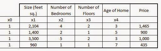
The Normal Equation Method: The exists a method in Linear Algebra where the concept of Metrices and Vectors are used to calculate the parameters $\theta_0$ and $\theta_1$ with iteration. This method is an efficient one, except in the case of very large datasets where it becomes computationally expensive due to the calculation of inverse of very large metrices.

To use the Normal Equation method of solving for $\theta_0$ and $\theta_1$ , the dataset has to be represented in a Matrix format.

Linear Regression : Understanding the Cost Function

Defining the Cost:

When we fit a regression line through an existing data, the line passes through the data and not all points will lie on the line (which will be the case for a perfect correlation between X and Y). There will be some points which are above the line and which are below the line.

The whole idea of regression is to fit the regression line such that the distance between the existing data points and the regression line is minimum (not the orthogonal distance, but the distance from the line measured in parallel to y axis as shown in the above figure). The points above the line would yield positive distance while the points below the line would yield negative distances.

The residual e is defined as $\hat {y_i}{-}{y_i}$

The errors are squared to eliminate negative values, and the Sum of Squared Erros (SSE) is minimized to obtain the coefficients of X in the equation $y=\theta_0+\theta_1{x}+e$

${SSE} = \sum_{i=1}^{m}{(\hat {y_i}{-}{y_i})}^2$

This method is known as Ordinary Least Squares (OLS)

The Hypothesis $h_\theta{(x)}$ is written as

 $h_{\theta}(x)={\theta_0}+{\theta_1}(x)$



The Cost Function (J) is typically written as
$J(\theta_0,\theta_1)={\frac{1}{2m}}\sum_{i=1}^m{({h_\theta}(x^{(i)})-y^{(i)})}^2$

The goal of the regression analysis is to minimize the coefficients $\theta_0$ and $\theta_1$ for a univariate regression. For Multivariate, there will be multiple variables for X ($x_1,x_2,x_3..$) with their respective coefficients ($\theta_1, \theta_2, \theta_3....$.) The coefficient term $\theta_0$ is the constant term in this equation.
--------------------------------------------------------------------------------------------------
To summarize:
Hypothesis: $h_{\theta}(x)={\theta_0}+{\theta_1}(x)$
Parameters: $\theta_0,\theta_1$
Cost Function:

$J(\theta_0,\theta_1)={\frac{1}{2m}}\sum_{i=1}^m{({h_\theta}(x^{(i)})-y^{(i)})}^2$

Goal: Minimize $J_{\theta_0,\theta_1}(\theta_0,\theta_1)$
--------------------------------------------------------------------------------------------------

Linear Regression : The Basics

Some Definitions of Linear Regression:

• When a player plays well in the team, the team always wins. Given that the player in the next match has played well, its highly probable that the team will win again
• Predicting the value of a variable by observing its relationship with another variable.
• Wiki :  Linear Regression is an approach for modeling the relationship between a scalar dependent variable y and one or more explanatory variables (or independent variable) denoted X
• Example: Price of a house is dependent on its area and number of bedrooms. Given the data about area of house and number of bedrooms (X: area(x1) & num_bedrooms(x2)) and their price (Y), find a relationship between Price of house and its area & number of bedrooms. Now, if you get a house's area and number of bedrooms, predict the price of tha house based on the historical data

All the above statements and examples are from the Supervised Learning paradigm of Machine Learning. They take some initial data, understand the pattern in it, and use the pattern on the new data to figure out the outcome

The Predictor variables (X) are known as predictors of independent variables, since they are independent and their values can change without being affected by any other variable

The Outcome Variable (Y) is known as dependent variable since its value is 'dependent' of the value of independent variables (X's), and if any of the X's change, the value of Y will have to change.

An equation is typically written as 

y: Outcome Variable

X: vector of Predictor variables (independent variables)

$\epsilon$: error term

$\beta$: Coefficient of the terms

Another way of representing the model is :

The Training Dataset goes into a learning model, which proposes a hypothesis 'h' which is used to take independent variables (X's) as input and produce a result (Outcome variable/Dependent Variable)

What is there is no relationship? Or how accurate is our model? How to measure it? What is the error term?  - All models come with a cost function which estimates the difference between the actual values of y's in the training data, and the gap with the prediction model. This gap between actual and estimated values of Ys is known as the Cost.

All optimization objectives are aimed at reducing the cost. Lesser the cost, better is the model (however there are other factors too).

Machine Learning : Some Interesting Use Cases

Some Interesting Use Cases (there are many many many more)...

• Identifying the pictures of humans from their and their friends on Facebook (automatic tagging)
• Going through videos on YouTube and identifying the cat videos
• Self Driven Cars
• Email SPAM detection (a pretty standard problem)
• Handwriting recognition
• Understanding Music Genre
• Recommendation Engine for Netflix and Amazon
• ...and many more

Looks Interesting !! The possibilities are endless !!

What language should be used for Machine Learning?

R vs. Python vs Matlab vs ....

Use anything you are comfortable with. The objective should not be to learn a language or learning machine learning in a standard language, but to understand the algorithm behind the solution.

There are a lot of tools (like Weka) which can run your models or packages in R or Python which take in the data and throws out the output, but make sure you understand the algorithm properly else you will not be able to tweak the model or improve its accuracy.

Open Source: R, Python, Octave
Paid: SAS, MATLAB

... plus a lot of other tools and platforms. Stick to one or two, and practice a lot.

If your aim is to go a level up, participate in Kaggle.com to know what type of problems are being solved by the top data scientists of the world. If you are just a business analyst who just ran some predictive models in R/SAS/SQL and analyzed some data, you will understand how much there is is still to learn !! 

The Need for Machine Learning

Why is it needed?

1. Too much data, and too many things that can be done with the help of this data which is not being done currently. A great opportunity in each and every field.
2. Machine Learning is not a subject in itself, it is always associated with some domain (inface most of the domains which have data can leverage this). Its actually 'Machine Learning for Retail' or 'Machine Learning for Media' or 'Machine Learning for Bioinformatics' or 'Machine Learning for Astronomy'. The possibilities are endless.
3. Imagine you have an e-commerce store and 10 customers buy from you (just saying). You know what each customer is like and what they prefer to buy in your head. What if you become hugely successful and the number of customers go up to 10 Million? Also the number of products you are selling go up to 100,000. There is no way you can make use of this data without using some advanced technologies.
4. Its not Rocket Science : Well, you are not developing a system like the Skynet or the Matrix (in that case, it is much more than Rocket Science). With dedicated effort, you can master the algorithms and use them with your own data in your own field. Most of the algorithms are not dependent on the domain (but their interpretation is). 
5. Availability of Technology : 10 years back, if you wanted to analyze 100GB of data, you had to make a lot of investments in the tools like SAS or buying up huge amount of server space just to store the data. With the advent of OpenSource Technologies like Hadoop, Hive, Pig etc, OpenSource and free programming languages like R, Python, Octave etc and utilizing cloud technologies, you probably just need a good computer to run your Machine Learning Algorithms.
6. Huge Scope: Data Scientist is the sexiest job of the 21st century. If you want to remain relevant in the job market, you need to learn Machine Learning to become a data scientist.

Having said all this, its not easy. A lot of effort, dedication and practice is required to master this. It seems difficult at first, then a bit easy, then insanely difficult and once you understand everything it becomes insanely easy.

Machine Learning : Supervised vs Unsupervised Learning

Machine Learning : Training computers to solve a problem without giving explicit instructions !

Everybody remembers the movie 'Terminator' and 'The Matrix'. Both movies take the idea of 'Artificial Intelligence' and show the extreme end of the spectrum. The computers in the movies (Skynet and the Matrix) somehow become so intelligent that they try to take control of the human civilization leading to a war between Man and Machine.

Ok, Lets skip the hypothetical (??) scenarios. Can computers really become so intelligent? We'll see. But there is a huge area of 'training' them to perform a task in a better and faster way than humans. And this area can be called a 'Machine Learning' or even 'Artificial Intelligence'

More Robust Definition : A computer program is said to learn from experience E with respect to some task T  and some performance measure P,  if its performance on T, as measured by P, improves with experience E.

Supervised Learning :  When the computer is provided with some data to train itself, and then it uses the training to apply the same model to a new and unseen data. Examples would include Linear and Logistic Regressions, Neural Networks, and SVMs.

Unsupervised Learning : When the computer is given the data and it applies some algorithm to understand the pattern in the data without the need of an explicit training. An example would be to give a list of data points in a 2-D plane and applying k-means clustering on the data.

There are a lot of factors, parameters and optimization that goes into the actual application and making sure the results are coming out as intended. After all, the computers are also an invention of human mind :)

An interesting example : The Cocktail Party Problem

The solution is just a one line code in MATLAB :)

Test Post & Disclaimer

Testing the layout and the page settings

Disclaimer: A lot of this information is from Professor. Andrew NG's awesome course in Machine Learning at Stanford, and I give full credit to him for teaching such a difficult concept in an easy way. Though I might not mention his name, a lot of material in this blog has been shamelessly lifted from his course.

If you want to do a proper course, please do this 10 week course at coursera by Prof. Andrew NG


Cheers !!!