Neural networks : Cost Function

Neural Network Classification:

Above: A Neural Network with 4 layers

Input Unit:  $\{ (x^{(1)},y^{(1)}),(x^{(2)},y^{(2)}),(x^{(3)},y^{(3)}),.,.,.,.,(x^{(m)},y^{(m)})\}$
L = Total number of layers in the network (L=4 in the above case)
$s_l$ = number of units (not counting bias units) in the layer $l$

There are two types of Neural Network outcomes:

Binary Classification:
$y$ = 0 or 1 ; 1 Output Unit
$s_L=1$, K=1

Multiclass Classification:

Number of output units: K

$y\in\Re^{(k)}$

E.g. if K=4

Output will be K vectors: $\begin{bmatrix}1 \cr 0\cr0\cr0\cr\end{bmatrix}$, $\begin{bmatrix}0 \cr 1\cr0\cr0\cr\end{bmatrix}$,$\begin{bmatrix}0\cr 0\cr1\cr0\cr\end{bmatrix}$,$\begin{bmatrix}0\cr 0\cr0\cr1\cr\end{bmatrix}$



Cost Function:

Cost function for a Neural Network is a generalization of the Cost Function of a Logistic Regression.

Logistic Regression Cost Function:

$J(\theta) = -\frac 1 m \left[\sum^m_{i=1}{y^{(i)}log(h_\theta(x^{(i)})+(1-y^{(i)})log(1-h_\theta(x^{(i)}))}\right] + \frac \lambda {2m} \sum_{j=1}^n\theta_j^2 $

Neural Network Cost Function:

Neural Network outputs vectors in $\Re^K$

$h_\Theta(x)\in \Re^K$;
$(h_\Theta(x))_i = i^{th}\  output$

Cost Function:
$J(\Theta) = -{\frac 1 m} \left[ {\sum_{i=1}^m}{\sum_{k=1}^K}{y_k^{(i)}log(h_\Theta(x)^{(i)})_k}\ +\
{(1-y_k^{(i)})log(1-(h_\Theta(x)^{(i)})_k)}
\right]\ + \
{\frac \lambda {2m}}{\sum_{l=1}^{L-1}}{\sum_{i=1}^{s_l}}{\sum_{j=1}^{s_{l+1}}}
(\Theta_{ji}^{(l)})^2
$

The Summation ${\sum_{k=1}^K}$ is over the 'K' output units i.e. summing the cost function for each of the output units K.

Regularization Term : We don't sum over the terms corresponding to the bias units $a_0$, corresponding to $\Theta_{i0}x_0$. Even if we include the bias terms, it will output similar result.

Logistic Regression :Cost Function & Gradient Descent

Logistic Regression: Cost Function

The Logistic Regression hypotheses function is given by
$h_\theta(x) = \frac 1 {1+e^{-\theta^Tx}}$

The question is : how do we choose the parameters $\theta$?

Recap: Linear Regression Cost Function

$J(\theta) = \frac 1 m \sum^m_{i=1} \frac 1 2 (h_\theta(x^{(i)}) - y^{(i)})^2$

Logistic Regression Cost Function:

In Logistic Regression, $h_\theta(x) = \frac 1 {1+e^{-\theta^Tx}}$  as opposed to linear regression where $h_\theta(x) = \theta_0 + \theta_1x_1...$.

The problem with representing the cost function of Logistic regression as $\frac 1 2 (h_\theta(x^{(i)}) - y^{(i)})^2$ is that the curve of $J(\theta)$ is a non convex one, i.e. it has multiple local minima which cannot be optimized by the Gradient Descent function. For Gradient Descent to converge, the cost function has to be a convex function as is the case with Linear Regression.

Cost Function :

$Cost (h_\theta(x),y) = -log(h_\theta(x))$ if y = 1

$Cost (h_\theta(x),y) = -log(1- h_\theta(x))$ if y = 0

or 

$Cost (h_\theta(x),y) = -ylog(h_\theta(x)) -(1-y)log(1- h_\theta(x))$

If y=1:

Cost = 0 if y=1 and $h_\theta(x)$ = 1 (i.e. if the actual value of y = 1 and the predicted value of y is also 1)

But as $h_\theta(x) \rightarrow 0$, $Cost \rightarrow \infty$

If y=0:

Cost = 0 if y=0 and $h_\theta(x)$ = 0 (i.e. if the actual value of y = 0 and the predicted value of y is also 0)

But as $h_\theta(x) \rightarrow 1$, $Cost \rightarrow \infty$

Simplified Cost Function:

$J(\theta) = \frac 1 m \sum^m_{i=1}Cost(h_\theta(x^{(i)}) - y^{(i)})^2$

$J(\theta) = -\frac 1 m \sum^m_{i=1}{y^{(i)}log(h_\theta(x^{(i)})+(1-y^{(i)})log(1-h_\theta(x^{(i)}))}$

Now, to fit parameters $\theta$, we need to minimize $J(\theta)$

To make a prediction given a new $x$:

Output $h_\theta(x) = \frac 1 {1+e^{-\theta^Tx}}$

Gradient Descent Function for Logistic Regression:

Pseudocode : repeat until convergence $\{$

$\theta_j := \theta_j - {\alpha}{\frac {\partial }{ \partial {\theta_j}}}{J(\theta)}$

$\}$

Putting in the value of the Cost Function:

$\theta_j : \theta_j-\alpha {\frac{1}{m}}\sum_{i=1}^m{({h_\theta}(x^{(i)})-y^{(i)})}.{x^{(i)}_j}$ Simultaneously update for all $\theta_j$

The algorithm of Gradient Descent for Logistic Regression is same as that for linear regression, the only difference is the value of $h_\theta(x)$ which in this case is $h_\theta(x) = \frac 1 {1+e^{-\theta^Tx}}$ instead of $h_\theta(x) = \theta^Tx$ for Linear Regression.

Cost Function : Multivariate Linear Regression

The concepts for calculating the cost function J, and estimating the parameters $\theta_0$ and $\theta_1$ can be easily extended to the case where we have multiple features in the dataset, i.e. instead of only one variable $x$ we have multiple variables $x_1, x_2, x_3...$ and so on.

Notations:

Consider a training dataset with 5 variables $x_1, x_2, x_3, x_4 and x_5$. The outcome variable is still $y$. There are $m$ examples in the dataset (number of rows)

$n$ = number of features
$x^{(i)}$ = input (features) of the $i^{th}$ training example
$x^{(i)}_j$ = value of feature $j$ in $i^{th}$ training example
Linear Regression : Multivariate [Multiple features]

Hypothesis:
Univariate: $h_{\theta}(x) = \theta_0 +\theta_1x$
Multivariate: $h_{\theta}(x) = \theta_0 +\theta_1x_1 + \theta_2x_2 +\theta_3x_3 +\theta_4x_4 ..... +\theta_nx_n  $

For convenience of notation, define $x_0$ =1

 $h_{\theta}(x) = \theta_0x_0 +\theta_1x_1 + \theta_2x_2 +\theta_3x_3 +\theta_4x_4 ..... +\theta_nx_n  $

The vector X contains $[x_0, x_1,x_2......x_n]$ and is a vector of dimension (n+1)
The vector $\theta$ contains $[\theta_0, \theta_1, \theta_2......\theta_n]$ and is a vector of dimension (n+1)

The hypothesis can be written as

$h_\theta(x) = \theta^TX$

Cost Function & Gradient Descent Algorithm for a Multivariate Linear Regression

Cost Function
$J(\theta_0,\theta_1,\theta_2.....\theta_n) = {\frac 1 {2m}}{\sum_{i=1}^m}{(h_\theta(x^{(i)})-y^{(i)})}^2$

Gradient Descent for $\theta_0,\theta_1,\theta_2....\theta_n$
repeat until convergence $\{$

$\theta_j : \theta_j-\alpha {\frac{1}{m}}\sum_{i=1}^m{({h_\theta}(x^{(i)})-y^{(i)})}.{x^{(i)}_j}$

$\}$ Simultaneously update $\theta_j$ for j= 0,1,....n


The value of $x_0$ is always 1, so this generalizes the Gradient Descent Algorithm for univariate as well as multivariate linear regression

Linear Regression : Understanding the Cost Function

Defining the Cost:

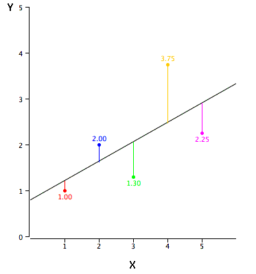
When we fit a regression line through an existing data, the line passes through the data and not all points will lie on the line (which will be the case for a perfect correlation between X and Y). There will be some points which are above the line and which are below the line.

The whole idea of regression is to fit the regression line such that the distance between the existing data points and the regression line is minimum (not the orthogonal distance, but the distance from the line measured in parallel to y axis as shown in the above figure). The points above the line would yield positive distance while the points below the line would yield negative distances.

The residual e is defined as $\hat {y_i}{-}{y_i}$

The errors are squared to eliminate negative values, and the Sum of Squared Erros (SSE) is minimized to obtain the coefficients of X in the equation $y=\theta_0+\theta_1{x}+e$

${SSE} = \sum_{i=1}^{m}{(\hat {y_i}{-}{y_i})}^2$

This method is known as Ordinary Least Squares (OLS)

The Hypothesis $h_\theta{(x)}$ is written as

 $h_{\theta}(x)={\theta_0}+{\theta_1}(x)$



The Cost Function (J) is typically written as
$J(\theta_0,\theta_1)={\frac{1}{2m}}\sum_{i=1}^m{({h_\theta}(x^{(i)})-y^{(i)})}^2 $

The goal of the regression analysis is to minimize the coefficients $\theta_0$ and $\theta_1$ for a univariate regression. For Multivariate, there will be multiple variables for X ($x_1,x_2,x_3..$) with their respective coefficients ($\theta_1, \theta_2, \theta_3....$.) The coefficient term $\theta_0$ is the constant term in this equation.
--------------------------------------------------------------------------------------------------
To summarize:
Hypothesis: $h_{\theta}(x)={\theta_0}+{\theta_1}(x)$
Parameters: $\theta_0,\theta_1$
Cost Function:

$J(\theta_0,\theta_1)={\frac{1}{2m}}\sum_{i=1}^m{({h_\theta}(x^{(i)})-y^{(i)})}^2 $

Goal: Minimize $J_{\theta_0,\theta_1}(\theta_0,\theta_1)$
--------------------------------------------------------------------------------------------------