Implementation Summary : Neural Networks

Training a Neural network:

Pick a network architecture (connectivity pattern between neurons)

No. of input units: Dimension of features $x^{(i)}$
No. of output units: Number of classes

Reasonable default: 1 hidden layer, or if >1 hidden layer, have same no. of hidden units in every layer (usually the more the better)

Training:

1. Randomly initialize weights
2. Implement forward propagation to get $h_\Theta(x^{(i)})$ for any $x^{(i)}$
3. Implement code to calculate the cost function $J(\Theta)$
4. Implement Backpropagation to compute partial derivatives $\frac \partial {\partial\Theta_{jk}^{(l)}}$

for i = 1 to m

     Perform forward propagation and backpropagation  using examples $(x^{(i)},y^{(i)})$

     (Get activations $a^{(l)}$ and delta terms $\delta^{(l)}$ for $l=2,3,4....,L$

     Calculate $\Delta^{(l)}:=\Delta^{(l)} + \delta^{(l+1)}(a^{(l)})^T

     ...

end;

Compute $\frac \partial {\partial\Theta_{jk}^{(l)}}J(\Theta)$

     5.  Use Gradient Checking to compare  $\frac \partial {\partial\Theta_{jk}${(l)}}J(\Theta)$ computed using backpropagation  vs. using numerical estimate  of gradient of $J(\Theta)$

     6.  Use Gradient Descent or advanced optimization method  with backpropagation  to try  to minimize $J(\Theta)$ as a function of parameters $\Theta$

Neural Networks: Unrolling Parameters, Gradient Checking & Random Initialization

Neural Networks: Unrolling Parameters

We need to unroll parameters from matrices to vectors to use in our optimization function like fminunc in Matlab/Octave

Advanced Optimization Functions:

function[jVal, gradient] = costFunction(theta);
...
optTheta = fminunc(@costFunction, initialTheta, options);

The above function assumes that the parameters initialTheta are vectors, not matrices. In Logistic regression, these parameters are vectors. However, in a Neural Network, these are matrices

For a Neural Network with 4 Layers (L=4)
$\Theta^{(1)}, \Theta^{(2)}, \Theta^{(3)}$ - matrices (Theta1, Theta2, Theta3)
$D^{(1)}, D^{(2)}, D^{(3)}$ = matrices (D1, D2, D3)

"Unroll into Vectors"

Example: lets say we have a 3 layer NN with the following details:
$s_1 = 10, s_2 = 10, s_3 = 1$

The dimension of matrices $\Theta$ and $D$ are given by:

$\Theta^{(1)}\in\Re^{10\times11}$, $\Theta^{(2)}\in\Re^{10\times11}$, $\Theta^{(3)}\in\Re^{1\times11}$

$D^{(1)} \in \Re^{10\times11}$, $D^{(2)} \in \Re^{10\times11}$, $D^{(3)} \in \Re^{1\times11}$

The command below will convert the matrices into vectors after combining them:
thetaVec = [Theta1(:);Theta2(:);Theta3(:)];
DVec = [D1(:);D2(:);D3(:)]

To recombine the vectors in the matrices in the initial format,
Theta1 = reshape(thetaVec(1:110),10,11);
Theta2 = reshape(thetaVec(111:220),10,11);
Theta3 = reshape(thetaVec(221:231),1,11);

Learning Algorithm:

Here is how we use the unrolling algorithm:

Have initial parameters $\Theta^{(1)},\Theta^{(2)},\Theta^{(3)}$
Unroll to get initialTheta  to pass to fminunc(@costFunction, initialTheta,options);

function [jVal,gradientvec] = costFunction(thetaVec);

• From thetaVec, get  $\Theta^{(1)},\Theta^{(2)},\Theta^{(3)}$ (reshape to get the original matrices back)
• Use forward propagation/back propagation to compute $D^{(1)}, D^{(2)}, D^{(3)}$ and $J(\Theta)$
• Unroll $D^{(1)}, D^{(2)}, D^{(3)}$ to get gradientVec

Numerical Gradient Checking:

The backpropagation algorithm is a bit complex, and even though the cost function J might seem to be decreasing, there could be a bug in the algorithm which could give erroneous results. The NN might end up with a high value of J.

How to check the gradient: Numerical Estimation of gradients (Gradient Checking)

We approximate the partial derivative of the function $J(\Theta)$, which is defined as the slope of the curve at that value of $\Theta$ by calculating the slope in a more geometrical way.

We select a point $\Theta+\epsilon$ just ahead of $\Theta$, and a point $\Theta-\epsilon$ just less than $\Theta$. The slope of the line connecting the values of $J(\Theta)$ at these points is given by the equation:

slope at $J(\Theta) = \frac {J(\Theta+\epsilon)-J(\Theta-\epsilon)}{2\epsilon}$

The value of $\epsilon \ approx 10^{-4}$


Implementation in Matlab or Octave:
gradApprox = (J(theta+EPSILON) - J(theta - EPSILON))/(2*EPSILON)

This will give a numerical estimate of slope at this point.

General case : Parameter vector $\theta$
$\theta \in \Re^n$ E.g. $\theta$ is 'unrolled' version of $\Theta^{(1)},\Theta^{(2)},\Theta^{(3)}...$
$\theta = \theta_1, \theta_2, \theta_3...\theta_n$

The partial derivatives of each of $\theta_1, \theta_2...\theta_n$ are calculated separately.

In Matlab/Octave, the following equation is implemented:
for i = 1 to n;
     thetaPlus = theta;
     thetaPlus(i) = thetaPlus(i) + EPSILON;
     thetaMinus = theta;
     thetaMinus(i) = thetaMinus(i) - EPSILON;
     gradApprox(i)  = (J(thetaPlus) - J(thetaMinus))/(2*EPSILON)
end;

Check that gradApprox $\approx$ DVec. If the values are very close, then we will be more confident that the algorithm is calculating the cost function J correctly and we will correctly optimize $\Theta$.

Implementation Note:

• Implement Backprop to compute DVec (unrolled $D^{(1)}, D^{(2)}, D^{(3)}$)
• Implement Numerical Gradient Checking to calculate gradApprox
• Make sure they give similar values
• Turn off gradient checking. using backprop code for learning

Important:

• Be sure to disable your code before training your classifier. if you run numerical gradient computation on every iteration of gradient descent ( or in the inner loop of the costFunction, your code will be very slow).

Random Initialization of $\Theta$:

Initial value of $\Theta$

What if we set all values of initialTheta = zeros(n,1)? The values of $\Theta$ determine the values in the activation units in each layer. In case the values are same, the cost function will not decrease as the partial derivaties of the cost function will be the same, so will the values of $\delta$ and $a_1,a_2...a_n$

After each update, the parameters corresponding to inputs going into each of the two hidden units are identical.

Random Initialization : Symmetry breaking

Initialize each $\Theta_{ij}^{(l)}$ to a random variable in $[-\epsilon,\epsilon]$, (i.e. $-\epsilon\le\Theta_{ij}^{(l)}\le\epsilon$)

E.g.:

Theta1 = rand(10,11) *(2*INIT_EPSILON)-INIT_EPSILON;

Theta2 = rand(1,11) *(2*INIT_EPSILON)-INIT_EPSILON;

rand(10,11) will give a random 10x11 matrix between 0 and 1;

Neural Networks: BackPropagation Algorithm

Gradient Computation:

The cost function for a Neural Network: We need to optimize the values of $\Theta$.

$J(\Theta) = -{\frac 1 m} \left[ {\sum_{i=1}^m}{\sum_{k=1}^K}{y_k^{(i)}log(h_\Theta(x)^{(i)})_k}\ +\ {(1-y_k^{(i)})log(1-(h_\Theta(x)^{(i)})_k)} \right]\ + \ {\frac \lambda {2m}}{\sum_{l=1}^{L-1}}{\sum_{i=1}^{s_l}}{\sum_{j=1}^{s_{l+1}}} (\Theta_{ji}^{(l)})^2$

Goal: $min_\Theta \ J(\Theta)$

We need to write the code to compute:

- $J(\Theta)$

- $\frac \partial {\partial\Theta_{ij}^{(l)}} J(\Theta)$

$\Theta_{ij}^l \in \Re$

How to compute the Partial Derivative Terms?

Example : Given One Training Example: Forward Propagation

Given one training example (x,y):

Forward Propagation: Vectorized implementation to calculate the activation values for all layers

$a^{(1)} = x$

$z^{(2)} = \Theta^{(1)}a^{(1)}$ 

$a^{(2)} = g(z^{(2)}) \ \ (add \ a_0^{(2)})$

$z^{(3)} = \Theta^{(2)}a^{(2)}$

$a^{(3)} = g(z^{(3)})\ \ (add\  a_0^{(3)})$

$z^{(4)} = \Theta^{(3)}a^{(3)}$

$a^{(4)} = h_\Theta(x) = g(z^{(4)})$

Gradient Computation: Backpropagation Algorithm

Intuition : We need to compute  $\delta_j^{(l)}$  which is the "error" of node $j$ in layer $l$, or error in the activation values

For each output unit (Layer L=4)

$\delta_j^{(4)} = a_j^{(4)} - y_j$ [$a_j^{(4)} = (h_\Theta(x))_j]$

This $\delta_j^{(4)}$ is essentially the difference between what out hypothesis outputs, and the actual values of y in our training set.

Writing in vectorized format:

$\delta^{(4)} = a^{(4)}-y$

Next step is to compute the values of $\delta$ for other layers.

$\delta^{(3)} = (\Theta^{(3)})^T\delta^{(4)}\ .* g'(z^{(3)})$

$\delta^{(2)} = (\Theta^{(2)})^T\delta^{(3)}\ .* g'(z^{(2)})$

There is no $\delta^{(1)}$ because the first layer correspond to the input units which asre used as such, and there is no error terms associated with it.

$g'()$ is the derivative of the sigmoid activation function.

It can be proved that $g'(z^{(3)}) = a^{(3)} .* (1-a^{(3)})$. Similarily, $g'(z^{(2)}) = a^{(2)} .* (1-a^{(2)})$

Finally, $\frac \partial {\partial\Theta_{ij}^{(l)}} J(\Theta) = a_j^{(l)}\delta_i^{(l+1)}$ (Ignoring $\lambda$; or $\lambda$=0)

Backpropagation Algorithm:

The name Backpropagation comes from the fact that we calculate the $\delta$ terms for the output layer first and then use it to calculate the values of other $\delta$ terms going backward.

Suppose we have a training Set: $\{(x^{(1)},y^{(1)}), (x^{(2)},y^{(2)}),.,.,.,.,(x^{(m)},y^{(m)})\}$

First, set $\Delta_{ij}^{(l)} = 0$ for all values of $l,i,j$ - This is used to compute $\frac \partial {\partial\Theta_{ij}^{(l)}} J(\Theta)$. Eventually, this  $\Delta_{ij}^{(l)}$ will be used to calculate the partial derivative  $\frac \partial {\partial\Theta_{ij}^{(l)}} J(\Theta)$. $\Delta_{ij}^{(l)}$  are used as accumulators.

For $i = 1\  to\  m$

     Set $a^{(1)} = x^{(i)}$ --> Activation for input layer

     Perform Forward Propagation to compute $a^{(l)}$ for $l = 2,3,...L$

     Using $y^{(i)}$, compute the error term for the output layer $\delta^{(L)} = a^{(L)}-y^{(i)}$

     Use backpropagation algorithm for computing $\delta^{(L-1)}, \delta^{(L-2)}, \delta^{(L-3)},...., \delta^{(2)}$, there is no $\delta^{(1)}$

     Finally, $\Delta$ terms are used to accumulate these partial derivatives terms $\Delta^{(l)}_{ij}:= \Delta^{(l)}_{ij} + a_j^{(l)}\delta_i^{(l+1)}$. In vectorized format it can be written as (assuming $\Delta$, $a$ and $\delta$ are all matrices : $\Delta^{(l)}:=\Delta^{(l)} + \delta^{(l+1)}(a^{(l)})^T$ 

end;

$D_{ij}^{(l)} := {\frac 1 m}\Delta_{ij}^{(l)} + \lambda\Theta_{ij}^{(l)}\ if\ j\ne0$

$D_{ij}^{(l)} := {\frac 1 m}\Delta_{ij}^{(l)} \ \ \ \ \ \ \ \ \ \ \ \ if\ j=0$

Finally, we can calculate the partial derivatives as : $\frac \partial {\partial\Theta_{ij}^{(l)}} J(\Theta) = D_{ij}^{(l)}$

---------------------------------------------------------------------------------

Backpropagation Intuition with Example:

Mechanical steps of Backpropagation Agorithm

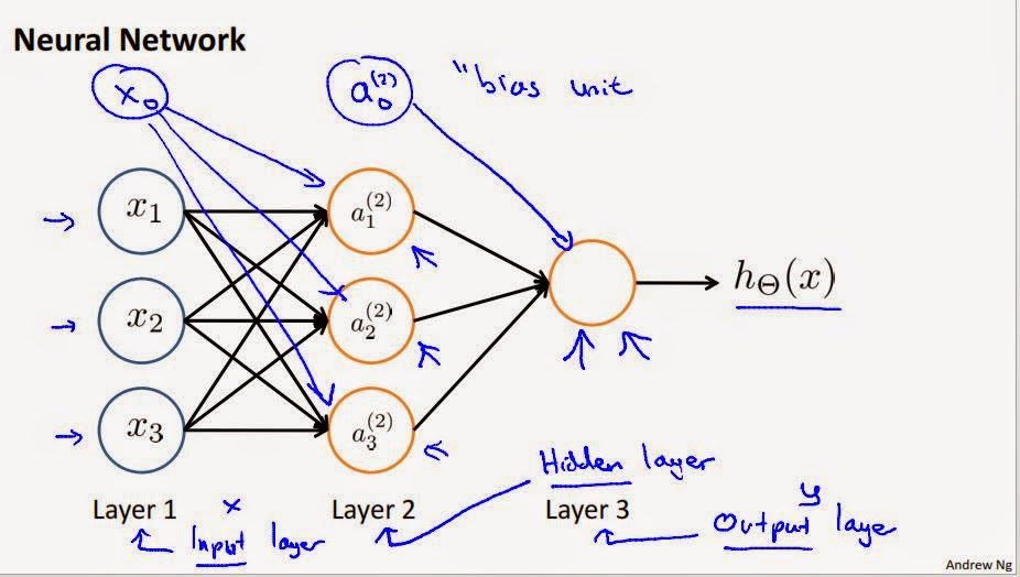
Forward Propagation: Consider a simple NN with 2 input units (not counting the bias unit), 2 activation unit in two layers (not counting bias unit in each layer) and one output unit in layer 4.

The input $(x^{(i)},y^{(i)}$ as represented as below. We first use Forward propagation to compute the values of $z_1^{(2)}$, and apply sigmoid activation function on $z_1^{(2)}$ to get the values of $a_1^{(2)}$. Similarly, the values of $z_2^{(2)}$ and $a_2^{(2)}$ are computed to complete the values of layer 2. The bias unit $a_0^{(2)} = 1$ is added to the layer 2.

Once the values of layer 2 are calculated, we apply the same methodology to compute the values of layer 3 (a & z)

For the values of Layer 3, we have values of $\Theta$ which is use to compute the values of $z_i^{(3)}$.

$z_1^{(3)} = \Theta_{10}^{(2)}a_0^{(2)} + \Theta_{11}^{(2)}a_1^{(2)} + \Theta_{12}^{(2)}a_2^{(2)}$

What is Backpropagation doing? Backpropagation is almost doing the same thing as forward propagation in the opposite direction (right to left, from output to input)

The cost function again:

$J(\Theta) = -{\frac 1 m} \left[ {\sum_{i=1}^m}{\sum_{k=1}^K}{y_k^{(i)}log(h_\Theta(x)^{(i)})_k}\ +\ {(1-y_k^{(i)})log(1-(h_\Theta(x)^{(i)})_k)} \right]\ + \ {\frac \lambda {2m}}{\sum_{l=1}^{L-1}}{\sum_{i=1}^{s_l}}{\sum_{j=1}^{s_{l+1}}} (\Theta_{ji}^{(l)})^2$

Assume $\lambda$ = 0 (remove the regularization term, ignoring for now).
Focusing on single example $x^{(i)},y^{(i)}$, the case of 1 output unit

cost($i$) = $y^{(i)}log\  h_\Theta(x^{(i)}) + (1-y^{(i)})log\  h_\Theta(x^{(i)})$ Cost associated with $x^i,y^i$ training example

Think of $cost (i) \approx  (h_\Theta(x^{(i)}) - y^{(i)})^2$ i.e. how well is the network doing on example (i) just for the purpose of intuition, how close is the output compared to actual observed values y

The $\delta$ terms are actually the partial derivatives of the cost associated with the example (i). They are a measure of how much the weights $\Theta$ needs to be changed to bring the hypothesis output $h_\Theta(x)$ closer to the actual observed value of y.

For the output layer, we first set the value of $\delta_1^{(4)} = y^{(i)}-a_1^{(4)}$. 

Next, we calculate the values of $\delta^{(3)}$ in the layer 3 using $\delta^{(4)}$, and the values of $\delta^{(2)}$ in the layer 2 using $\delta^{(3)}$. Please note that there is no $\delta^{(1)}$.

Focusing on calculating the value of $\delta_2^{(2)}$, this is actually the weighted sum (weights being the parameters $\Theta$ and the values of $\delta_1^{(3)}$ and $\delta_2^{(3)}$

$\delta_2^{(2)} = \Theta_{12}^{(2)}\delta_1^{(3)}+ \Theta_{22}^{(2)}\delta_2^{(3)}$
This corresponds to the magenta values + red values in the above diagram

Similarly, to calculate $\delta_2^{(3)}$,

$\delta_2^{(3)} =  \Theta_{12}^{(3)}\delta_1^{(4)}$

Once we calculate the values of $\delta$, we can use the optimizer function to calculate the optimized vaues of $\Theta$

Neural networks : Cost Function

Neural Network Classification:

Above: A Neural Network with 4 layers

Input Unit:  $\{ (x^{(1)},y^{(1)}),(x^{(2)},y^{(2)}),(x^{(3)},y^{(3)}),.,.,.,.,(x^{(m)},y^{(m)})\}$
L = Total number of layers in the network (L=4 in the above case)
$s_l$ = number of units (not counting bias units) in the layer $l$

There are two types of Neural Network outcomes:

Binary Classification:
$y$ = 0 or 1 ; 1 Output Unit
$s_L=1$, K=1

Multiclass Classification:

Number of output units: K

$y\in\Re^{(k)}$

E.g. if K=4

Output will be K vectors: $\begin{bmatrix}1 \cr 0\cr0\cr0\cr\end{bmatrix}$, $\begin{bmatrix}0 \cr 1\cr0\cr0\cr\end{bmatrix}$,$\begin{bmatrix}0\cr 0\cr1\cr0\cr\end{bmatrix}$,$\begin{bmatrix}0\cr 0\cr0\cr1\cr\end{bmatrix}$



Cost Function:

Cost function for a Neural Network is a generalization of the Cost Function of a Logistic Regression.

Logistic Regression Cost Function:

$J(\theta) = -\frac 1 m \left[\sum^m_{i=1}{y^{(i)}log(h_\theta(x^{(i)})+(1-y^{(i)})log(1-h_\theta(x^{(i)}))}\right] + \frac \lambda {2m} \sum_{j=1}^n\theta_j^2$

Neural Network Cost Function:

Neural Network outputs vectors in $\Re^K$

$h_\Theta(x)\in \Re^K$;
$(h_\Theta(x))_i = i^{th}\  output$

Cost Function:
$J(\Theta) = -{\frac 1 m} \left[ {\sum_{i=1}^m}{\sum_{k=1}^K}{y_k^{(i)}log(h_\Theta(x)^{(i)})_k}\ +\ {(1-y_k^{(i)})log(1-(h_\Theta(x)^{(i)})_k)} \right]\ + \ {\frac \lambda {2m}}{\sum_{l=1}^{L-1}}{\sum_{i=1}^{s_l}}{\sum_{j=1}^{s_{l+1}}} (\Theta_{ji}^{(l)})^2$

The Summation ${\sum_{k=1}^K}$ is over the 'K' output units i.e. summing the cost function for each of the output units K.

Regularization Term : We don't sum over the terms corresponding to the bias units $a_0$, corresponding to $\Theta_{i0}x_0$. Even if we include the bias terms, it will output similar result.

Neural Networks: MultiClass Classification

Neural Network: Model Representation

Anatomy of a Neuron:

A simgle neuron can be explained by the following system: Dendrites to collect information and transmit information, a cell body as a node/processing unit and Axon as an output wire

We can mimic a simple Logistic Model as a neuron by the following diagram:

The Output function $h_\theta(x)$ is defined by the sigmoid (logistic) activation function $\frac 1 {1+e^{-\theta^Tx}}$

The matrix of weights / parameters is defined by $\theta$ as $\begin{bmatrix}\theta_0 \cr \theta_1 \cr \theta_2 \cr \theta_3 \cr \end{bmatrix}$, the input vector $x$ is defined by $\begin{bmatrix}x_0 \cr x_1 \cr x_2 \cr x_3 \cr \end{bmatrix}$

Sigmoid (logistic) activation function:

$g(z) = \frac 1 {1+e^{-z}}$

The abovementioned representation is for a very simple and basic network with only one hidden layer having only one unit. Typically, a Neural Network has multiple input layer units, multiple hidden layers with multiple units, and multiple output units for multi-class classification.

The input layer has an additiona unit called 'The Bias Unit'($x_0$) which is equal to 1. The activation layers will also have an additional Biad Units equal to one.

Neural Network:

Details:

The Neural Network above consists of three layers : an Input Layer (Layer 1), a Hidden Layer (Layer 2), and an Output Layer (Layer 3). Both the Input and Hidden Layers (Layers 1 and 2) contain a bias unit $x_0$ and $a_0^{(2)}$ respectively.

The Hidden Layer: The Layer 2 or the 'Activation Layer' consists of xxactivation units $a_i^j$ which are defined by weight from the Input Layers. Each Input unit feeds to each Activation unit, and the interaction is characterized by the weight parameters $\theta$.

Number of Units: 4 (including a bias input unit) in  Layer 1, 4 (including a bias activation unit) in Layer 2, 1 in Output Layer (Layer 3).

Definitions:

$a_i^{(j)}$: Activation of unit $i$ in layer $(j)$;

$\Theta^{(j)}$: matrix of weights controlling the function mapping from layer $(j)$ to layer $(j+1)$.

$\Theta^{(1)}$ $\in$ $\Re^{3x4}$ : 3 rows for each activation unit $a_1^{(2}), a_2^{(2)}$ and $a_3^{(2)}$. The fourth unit in activation layer $a_0^{(2)}$  is the bias unit equal to 1. The rows 1 to 4 are for the input parameters (including the bias input unit) $x_0, x_1, x_2$ and $x_3$.

The subscript denotes the units (0,1,2, and 3), and the superscript denotes the layer number (1,2 or 3).

$a_1^{(2)}$ denotes the first unit in the second layer.

The sigmoid function $g(z)$ is defined by  $g(z) = \frac 1 {1+e^{-z}}$

z is defined as follows:

Layer 2: The activation layer

$a_1^{(2)}=g(\Theta_{10}^{(1)}x_0 + \Theta_{11}^{(1)}x_1 + \Theta_{12}^{(1)}x_2 + \Theta_{13}^{(1)}x_3)$

$a_2^{(2)}=g(\Theta_{20}^{(1)}x_0 + \Theta_{21}^{(1)}x_1 + \Theta_{22}^{(1)}x_2 + \Theta_{23}^{(1)}x_3)$

$a_3^{(2)}=g(\Theta_{30}^{(1)}x_0 + \Theta_{31}^{(1)}x_1 + \Theta_{32}^{(1)}x_2 + \Theta_{33}^{(1)}x_3)$

Layer 3: The output layer

$h_\Theta(x) = a_1^{(3)} = g(\Theta_{10}^{(2)}a_0^{(2)} + \Theta_{11}^{(2)}a_1^{(2)} + \Theta_{12}^{(2)}a_2^{(2)} + \Theta_{13}^{(2)}a_3^{(2)})$

Dimensions of $\Theta^{(j)}$: If the network has $s_j$ units in layer $j$, $s_{j+1}$ units in layer (j+1), then $\Theta^{(j)}$ will be of the dimension $s_{j+1}\times(s_j+1)$

The value of z:
$a_1^{(2)} = g(z_1^{(2)})$
$a_2^{(2)} = g(z_2^{(2)})$
$a_3^{(2)} = g(z_3^{(2)})$

$a_1^{(3)} = g(z^{(3)})$


Forward Propogation Model: Vectorized Implementation:

Define X, $\Theta$, $z_i^j$, $a_i^j$ in a vector notation

$x = \begin{bmatrix}x_0 \cr x_1 \cr x_2 \cr x_3 \cr \end{bmatrix} = \begin{bmatrix}a_0^{(1)} \cr a_1^{(1)} \cr a_2^{(1)} \cr a_3^{(1)}\cr \end{bmatrix}$

$a^{(1)} = x =$$\begin{bmatrix}x_0 \cr x_1 \cr x_2 \cr x_3 \cr \end{bmatrix} = \begin{bmatrix}a_0^{(1)} \cr a_1^{(1)} \cr a_2^{(1)} \cr a_3^{(1)}\cr \end{bmatrix}$

$\Theta^{(1)} = \begin{bmatrix} \Theta_{10}^{(1)} & \Theta_{11}^{(1)} & \Theta_{12}^{(1)} & \Theta_{13}^{(1)} \cr \Theta_{20}^{(1)} & \Theta_{21}^{(1)} & \Theta_{22}^{(1)} & \Theta_{23}^{(1)} \cr \Theta_{30}^{(1)} & \Theta_{31}^{(1)} & \Theta_{32}^{(1)} & \Theta_{33}^{(1)} \cr \end{bmatrix} \in \Re^{3\times4}$

$z^{(2)} = \Theta^{(1)}a^{(1)}$

$\Theta^{(1)} : 3\times 4$, $a^{(1)} : 4 \times 1$; $z^{(2)} : 3 \times 1$

$a^{(2)} = g(z^{(2)})$, $\in \Re^3$

Add $a_0^{(2)} = 0$ as a bias unit in activation layer (layer 2)

$\Theta^{(2)} = \begin{bmatrix} \Theta_{10}^{(2)} & \Theta_{11}^{(2)} & \Theta_{12}^{(2)} & \Theta_{13}^{(2)} \end{bmatrix} \in \Re^{1\times4}$

$z^{(3)} = \Theta^{(2)}a^{(2)}$

$\Theta^{(2)} : 1\times 4$, $a^{(2)} : 4 \times 1$; $z^{(3)} : 1 \times 1$

$h_\Theta(x) = g(\Theta_{10}^{(2)}a_0^{(2)} + \Theta_{11}^{(2)}a_1^{(2)} + \Theta_{12}^{(2)}a_2^{(2)} + \Theta_{13}^{(2)}a_3^{(2)})$

$h_\Theta(x) = a^{(3)} = g(z^{(3)})$


Neural Network learning its own features: Forward Propagation

This is called a forward propagation because we map the function from layer 1 to layer 2, establish the weight parameters, and then map the function from layer 2 to layer 3. Each layer and parameters $\Theta$ works as an input for the next layer, till it reaches the output layer.


Network Architecture: 

A Neural Network can be more complex than the one shown above. A Neural Network can have multiple activation layers $a^{(j)}$, and also multiple output layers.

Neural Networks: Introduction

Neural Networks: Introduction - How is it different from Logistic Regression

Neural Networks are a class of algorithms that is used widely for many purposes. It mimics the functioning of the brain (Neurons, hence the name) and try to simulate the network in the human brain to teach / train a computer.

Why not logistic regression: Logistic regression is also a class of algorithm pretty much used for solving similar set of problems as is the case with neural networks, but there are variour constraints with Logistic Regression. Logistic Regression is typically for a small set of features, where all the polynomial terms can be included in the model ($x_1^2x_2, x_1x_2^2$, etc). The problem occurs when we have too many features : what if we have 100 variables, and wee need every combination of all the variables which will include terms like $x_{23}^3x_{74}^7x_{12}^{33}$ and so on. It becomes extremely hard to create and analyze these features. Also, this will lead to the problem of overfitting, and these computations will be extremely computationally expensive. To solve this, if we reduce the number of features, we will lose information about the data.

Neural Networks aim to solve this issue. It is built to optimize for evaluating a huge number of features which is a typical case in any of the image recognition or handwriting recognition problem. It can be used for simple classification, multiclass classification or prediction models.

Regularization : Logistic Regression

Regularization: Logistic Regression

The problem of overfitting can occur in a Logistic regression model in case the model includes high order polynomial terms, like the following quation

$h_\theta(x) = g(\theta_0 +\theta_1x_1 + \theta_2x_1^2 + \theta_3x_1^2x_2 + \theta_4x_1^2x_2^2 + \theta_5x_1^2x_2^3... )$

The cost function of a Logistic Regression model is given by:

$J(\theta) = -\frac 1 m \sum^m_{i=1}{y^{(i)}log(h_\theta(x^{(i)})+(1-y^{(i)})log(1-h_\theta(x^{(i)}))}$

In a similar way as regularization using Linear Regression, we add a regularization term to the cost function which is defined as $\frac \lambda {2m} \sum_{j=1}^n\theta_j^2$

We do not add $\theta_0$ in the regularization term, and the regularization parameter is defined for $\theta_1, \theta_2, \theta_3.....\theta_n$

The Cost Function for Logistic regression becomes:

$J(\theta) = -\left[\frac 1 m \sum^m_{i=1}{y^{(i)}log(h_\theta(x^{(i)})+(1-y^{(i)})log(1-h_\theta(x^{(i)}))}\right] + \frac \lambda {2m} \sum_{j=1}^n\theta_j^2$

Gradient Descent with Regularization:
$\theta_0 := \theta_0-\alpha\left[ {\frac{1}{m}}\sum_{i=1}^m{({h_\theta}(x^{(i)})-y^{(i)})}.{x^{(i)}_j}\right]$

$\theta_j := \theta_j-\alpha\left[ {\frac{1}{m}}\sum_{i=1}^m{({h_\theta}(x^{(i)})-y^{(i)})}.{x^{(i)}_j} - \frac \lambda m \theta_j \right]$ Simultaneously update for all $\theta_j$

The value of $\theta_0$ is calculated separately without adding the regularization term. The value of j ranges from 1...n in the regularization term.

Regularization with Advanced Optimization:

Estimating $\theta$ using advanced optimization


Code:

function [jVal, gradient] = costFunction(theta)

jVal = [code to compute $J(\theta)$]

$J(\theta) = -\left[\frac 1 m \sum^m_{i=1}{y^{(i)}log(h_\theta(x^{(i)})+(1-y^{(i)})log(1-h_\theta(x^{(i)}))}\right] + \frac \lambda {2m} \sum_{j=1}^n\theta_j^2$

gradient(1) = [code to compute $\frac \partial {\partial\theta_0} J(\theta)$]

No regularization term for $\theta_0$

gradient(2) = [code to compute $\frac \partial {\partial\theta_1} J(\theta)$]

$\frac 1 m \sum_{i=1}^m (h_\theta(x^{(i)})-y^{(i)}).x_1^{(i)} - \frac \lambda m \theta_1$

gradient(3) = [code to compute $\frac \partial {\partial\theta_2} J(\theta)$]

$\frac 1 m \sum_{i=1}^m (h_\theta(x^{(i)})-y^{(i)}).x_2^{(i)} - \frac \lambda m \theta_2$

.

.

.

gradient(n+1) = [code to compute $\frac \partial {\partial\theta_n} J(\theta)$]

$\frac 1 m \sum_{i=1}^m (h_\theta(x^{(i)})-y^{(i)}).x_n^{(i)} - \frac \lambda m \theta_1$

Regularization : Linear Regression

Regularization : Linear Regression

$J(\theta)$ = $min \frac 1 {2m} \left[\sum_{i=1}^m {(h_\theta(x^{(i)})-y^{(i)})^2} + \lambda\sum_{j=1}^n\theta_j^2 \right]$

Goal: minimize $J(\theta)$

Gradient Descent:

GD Algorithm without the regularization term:

repeat until convergence $\{$

$\theta_0 := \theta_0 - \alpha{\frac{1}{m}}\sum_{i=1}^m{({h_\theta}(x^{(i)})-y^{(i)})}.x_0^{(i)}$

$\theta_j := \theta_j-\alpha {\frac{1}{m}}\sum_{i=1}^m{({h_\theta}(x^{(i)})-y^{(i)})}.{x_j^{(i)}}$

$\}$

Gradient Descent with Regularization term $\lambda$ added:

Since we are not regularizing $\theta_0$, it is updated separately and the regularization term is not included in the calculation of $\theta_0$

repeat until convergence $\{$

$\theta_0 := \theta_0 - \alpha{\frac{1}{m}}\sum_{i=1}^m{({h_\theta}(x^{(i)})-y^{(i)})}.x_0^{(i)}$

$\theta_j := \theta_j-\alpha \left[{\frac{1}{m}}\sum_{i=1}^m{({h_\theta}(x^{(i)})-y^{(i)})}.{x_j^{(i)}} - \frac \lambda m \theta_j \right]$
(j= 1,2,3,....n)
$\}$

Simplifying:

$\theta_j := \theta_j(1-\alpha\frac \lambda m) - \alpha\frac 1 m \sum_{i=1}^m{({h_\theta}(x^{(i)})-y^{(i)})}.{x_j^{(i)}}$


The term $(1-\alpha\frac \lambda m)$ is less than 1 (0.9 or 0.95) and this reduces the value of $\theta_j$ in every step by multiplying it repeatedly with a number less than 1, thus achieveing the goal of regularization.


Normal Equation Method:

Matrices:

X : m x (n+1) matrix
y:  m- dimensional vector

Without Regularization:

$\theta = (X^TX)^{-1}X^Ty$

With Regularization

$\theta = (X^TX + \lambda\begin{bmatrix}0& 0& 0& 0& 0& 0 \cr 0& 1& 0& 0& 0& 0 \cr 0& 0& 1& 0& 0& 0 \cr 0& 0& 0& .& .& . \cr 0& 0& 0& .& .& .\cr 0& 0& 0& .& .& 1\cr\end{bmatrix})^{-1}X^Ty$

The Matrix multiplied with $\lambda$ is a $(n+1)$ x$(n+1)$ matrix, where the first row, first columns and all other non diagonal elements are 0. Only the elements on the main diagonal (except the first one) are equal to 1

The Normal equation method with regularization takes care of the non-invertibility of the matrix $X^TX$

Regularization for Linear & Logistic Regression : Overfitting & Cost Function

The Problem of Over fitting:

The parameters that generate a model might throw up three type of results: Overfit, Right Fit and Underfit

Overfitting:

• High Variance scenario, the model fits too well with the training data
• Usually occurs due to the presence of large number of higher order parameters
• Fits the training examples quite well, but fails to generalize to new examples

Underfitting:

• High Bias scenario, the model fits poorly with the data and usually biased (generalized one result for all data)
• Doesn't fit the training data well

Addressing Overfitting:

1. Reduce the number of features
1. Manually Select which features to keep
2. Model selection algorithm
2. Regularization
1. Keep all the features, but reduce the magnitude/values of parameters $\theta_j$
2. Works well when we have a lot of features, each one of which contributes a bit in predicting $y$

 Regularization: Cost Function

Intuition:

$h_\theta(x)$ for an overfitted function :

$\theta_0 + \theta_1x + \theta_2x^2+\theta_3x^3+\theta_4x^4$

If we penalize and make $\theta_3$ and $\theta_4$ very small, by changing the cost function to:

Cost ($J(\theta)$) = $min \frac 1 {2m} \sum_{i=1}^m {(h_\theta(x)-y)^2} + 1000\theta_3^2 + 1000\theta_4^2$

Multiplying 1000 to $\theta_3$ and $\theta_4$ in the cost function forces the algorithm to reduce the value of both  $\theta_3$ and $\theta_4$ and make it very close to 0.

The smaller values of all $\theta$'s will generate a simpler hypothesis which will be less prone to overfitting.

Implementaion:

The Regularization Parameter $\lambda$:

 

The cost function can be rewritten as :

Cost ($J(\theta)$) = $min \frac 1 {2m} \left[\sum_{i=1}^m {(h_\theta(x^{(i)})-y^{(i)})^2} + \lambda\sum_{j=1}^n\theta_j^2 \right]$

Points to note:

• An extra term is added to regularize all the $\theta$ parameters, $\theta_0$ is not penalized (the summation term starts at j=1 and not at j=0, leaving $\theta_0$)
• The parameter $\lambda$ controls a tradeoff between two goals of the equation : Fit the data well (first part), and keep the coefficients small (second part)
• Selecting the value of $\lambda$: If $\lambda$ is too large, the parameters $\theta$ will be penalized very heavily and will become very close to 0. The hypothesis will become $h_\theta(x) = \theta_0$ which is a highly biased hypothesis
• If $\lambda$ is too large, the Gradient Descent Algorithm will fail to converge

Logistic Regression : One Vs All Classification

MultiClass Classification : Logistic Regression

Examples:

• Email Folder tagging: Work (y=1), Friends (y=2), Family (y=3), Travel (y=4)
• Weather : Sunny (y=1), Cloudy (y=2), Rain (y=3)

The outcome variable y is not restricted to only two outcomes $y=\pmatrix{0 \cr 1}$ but is defined by $y=\pmatrix{1 \cr 2 \cr 3 \cr 4\cr}$ depending on the number of classifications/ groups we need to make.

In the multiclass classification, we train the model separately for y=1, y=2, y=3 and so on, and for each outcome, we select the class that maximizes $h_\theta^{(i)}(x)$

$h_\theta^{(i)}(x) = P(y=i | x;\theta)$

Train a logistic regression classifier $h_\theta^{(i)}(x)$ for each class $i$ to predict the probability that $y=i$.

On a new input $x$, to make a prediction, pick the class $i$ that maximizes $h_\theta^{(i)}(x)$

Logistic Regression : Advanced Optimization

Advanced Optimization for Logistic Regression : Finding the values of $\theta$

Gradient Descent Algorithm is one way to calculate the value of parameters $\theta$. However, it involves selecting a appropriate value of $\alpha$ which might cause multiple iterations.

There are various other optimization algorithms available for minimizing a cost function $J(\theta)$ which are a bit more complex, but there is no need to manually pick a value of $\alpha$ and are much faster than Gradient Descent. The other algorithms are Conjugate Gradient, BFGS and L-BFGS.

Coding the Advanced Optimization Algorithms in MATLAB/Octave:

Example:

say we have to optimize $\theta_1 and \theta_2$, and $J(\theta)$ is given by
$J(\theta) = {(\theta_1-5)}^2+{(\theta_2-5)}^2$
$\frac \partial {\partial\theta_1} J(\theta) = 2(\theta_1-5)$
$\frac \partial {\partial\theta_2} J(\theta) = 2(\theta_2-5)$

We write the function in Matlab/Octave which calculates the value of the cost function $J(\theta)$ and the partial derivatives (gradient 1 for $\theta_1$ and gradient 2 for $\theta_2$)

Note: The index in Octave/Matlab starts from 1; so $\theta_0, \theta_1.....\theta_n$ in the equation is equal to $\theta_1, \theta_2,....\theta_{n+1}$

Code:
function[jVal, gradient] = costFunction(theta)

jVal = (theta(1)-5)^2 + (theta(2)-5)^2;
gradient = zeros(2,1)
gradient(1) = 2*(theta(1)-5)
gradient(2) = 2*(theta(2)-5)
....

Once the code for calculating jVal (the cost function) and gradient is written, the values of $\theta$ are optimized by the following code:

options = optimset('GradObj','on','MaxIter','100');
initialTheta = zeros(2,1)
[optTheta, functionVal, exitFlag]...
     = fminunc(@costFunction, intitalTheta,options);



Recap:

theta = $\pmatrix{\theta_0 \cr \theta_1 \cr .\cr .\cr \theta_{n}}$
function[jVal, gradient] = costFunction(theta)

jVal = [code to compute $J(\theta)$]

gradient(1) = [code to compute $\frac \partial {\partial\theta_0} J(\theta)$]
gradient(2) = [code to compute $\frac \partial {\partial\theta_1} J(\theta)$]

gradient(n+1) = [code to compute $\frac \partial {\partial\theta_n} J(\theta)$]

Logistic Regression :Cost Function & Gradient Descent

Logistic Regression: Cost Function

The Logistic Regression hypotheses function is given by
$h_\theta(x) = \frac 1 {1+e^{-\theta^Tx}}$

The question is : how do we choose the parameters $\theta$?

Recap: Linear Regression Cost Function

$J(\theta) = \frac 1 m \sum^m_{i=1} \frac 1 2 (h_\theta(x^{(i)}) - y^{(i)})^2$

Logistic Regression Cost Function:

In Logistic Regression, $h_\theta(x) = \frac 1 {1+e^{-\theta^Tx}}$  as opposed to linear regression where $h_\theta(x) = \theta_0 + \theta_1x_1...$.

The problem with representing the cost function of Logistic regression as $\frac 1 2 (h_\theta(x^{(i)}) - y^{(i)})^2$ is that the curve of $J(\theta)$ is a non convex one, i.e. it has multiple local minima which cannot be optimized by the Gradient Descent function. For Gradient Descent to converge, the cost function has to be a convex function as is the case with Linear Regression.

Cost Function :

$Cost (h_\theta(x),y) = -log(h_\theta(x))$ if y = 1

$Cost (h_\theta(x),y) = -log(1- h_\theta(x))$ if y = 0

or 

$Cost (h_\theta(x),y) = -ylog(h_\theta(x)) -(1-y)log(1- h_\theta(x))$

If y=1:

Cost = 0 if y=1 and $h_\theta(x)$ = 1 (i.e. if the actual value of y = 1 and the predicted value of y is also 1)

But as $h_\theta(x) \rightarrow 0$, $Cost \rightarrow \infty$

If y=0:

Cost = 0 if y=0 and $h_\theta(x)$ = 0 (i.e. if the actual value of y = 0 and the predicted value of y is also 0)

But as $h_\theta(x) \rightarrow 1$, $Cost \rightarrow \infty$

Simplified Cost Function:

$J(\theta) = \frac 1 m \sum^m_{i=1}Cost(h_\theta(x^{(i)}) - y^{(i)})^2$

$J(\theta) = -\frac 1 m \sum^m_{i=1}{y^{(i)}log(h_\theta(x^{(i)})+(1-y^{(i)})log(1-h_\theta(x^{(i)}))}$

Now, to fit parameters $\theta$, we need to minimize $J(\theta)$

To make a prediction given a new $x$:

Output $h_\theta(x) = \frac 1 {1+e^{-\theta^Tx}}$

Gradient Descent Function for Logistic Regression:

Pseudocode : repeat until convergence $\{$

$\theta_j := \theta_j - {\alpha}{\frac {\partial }{ \partial {\theta_j}}}{J(\theta)}$

$\}$

Putting in the value of the Cost Function:

$\theta_j : \theta_j-\alpha {\frac{1}{m}}\sum_{i=1}^m{({h_\theta}(x^{(i)})-y^{(i)})}.{x^{(i)}_j}$ Simultaneously update for all $\theta_j$

The algorithm of Gradient Descent for Logistic Regression is same as that for linear regression, the only difference is the value of $h_\theta(x)$ which in this case is $h_\theta(x) = \frac 1 {1+e^{-\theta^Tx}}$ instead of $h_\theta(x) = \theta^Tx$ for Linear Regression.

Logistic Regression: Decision Boundary

Logistic Regression : Decision Boundary

$h_\theta(x) = g(\theta^Tx)$

$g(z) = \frac 1 {1+e^{-z}}$

Threshold:

Predict y=1 if $h_\theta(x)\ge0.5$ or $\theta^Tx\ge0$
g(z) $\ge$ 0.5 when z $\ge$ 0
$h_\theta(x) = g(\theta^Tx)$

Predict y=0 if $h_\theta(x)\lt0.5$ or $\theta^Tx\lt0$
g(z) $\lt$ 0.5 when z $\lt$ 0
$h_\theta(x) = g(\theta^Tx)$

Decision Boundary:

Decision Boundary is the property of the hypothesis and the parameters, and not the property of the dataset

In the above example, the two datasets (red cross and blue circles) can be separated by a decision boundary whose equation is given by:

$h_\theta(x) = g(\theta_0 + \theta_1x_1 + \theta_2x_2)$

Suppose the parameters $\theta$ is defined by the vector

$\theta = \pmatrix {-3 \cr 1 \cr 1 \cr}$

The model becomes:

Predict "y=1" if $-3 + x_1 + x_2 \ge 0$
or $x_1 + x_2 \ge 3$

Similarily, Predict "y=0" if $x_1 + x_2 \lt 3$

At the Decision Boundary, when $x_1 + x_2 =3$, $h_\theta(x) = 0.5$

A Decision boundary can be nonlinear, depending on the parameters. For example, a logistic regression optimized by the following hypothesis will result in a circular Decision Boundary

$h_\theta(x)  = g(\theta_0 +  \theta_1x_1 + \theta_2x_2 + \theta_3x_1^2 + \theta_4x_2^2)$
where the vector $\theta$ is given by $\theta = \pmatrix{-1 \cr 0\cr0\cr1\cr1\cr}$

In this case, predict "y=1" when $z\ge0$, where $z=-1 +x_1^2+x_2^2$

The Cost Function  and the Gradient Descent Algorithm works much in the similar manner as the Linear Regressionm, with the exception of the function $h_\theta(x)$ which is different for Linear and Logistic Regression.

Classification using Logistic Regression

Classification using Logistic Regression:

Classification is different from linear regression as it classifies the data into two or more categories. It is still called regression as it takes the input from the training data and creates a model much like linear regression, but since it uses the Logit function to classify the data points, it is named Logistic Regression.

Why can't we use Linear Regression for Classification : Linear regression can be used to separate two sets of data points using a higher order polynomial (in case of non-linear decision boundary) but presence of any outlier seriously affects the classification when we use Linear Regression. This problem can be easily solved using Logistic Regression.

Logistic regression examples:

• Emails: Spam/Not Spam
• Online Transactions: Fraud/Not Fraud
• Tumor: Malignant/Benign

Typically the target variable (outcome) is classified as 

$y \epsilon \{0,1\}$

0: Negative Class (e.g. benign Tumor)

1: Positive Class (e.g. malignant tumor)

Differences with Linear Regression:

Logistic: y = 0 or 1

Logistic:$0\le h_\theta(x) \le 1$

Linear: $h_\theta(x)$ can be >1 or <0

Logistic Regression Model:

Want: $0\le h_\theta(x) \le 1$

$h_\theta(x) = g(\theta^Tx)$

$g(z) = \frac 1 {1+e^{-z}}$

where $z= \theta^Tx$

The function g(z) is also called the Logit function or the Sigmoid Function

Interpretation of Hypothesized Output:

$h_\theta(x)$ = estimated probability that y=1 on input x

Example: If $h_\theta(x)$ = 0.7, there is a 70% chance that y = 1

$h_\theta(x) = P(y=1 | x ; \theta)$

Linear Regression : Implementation using Normal Equation

Normal Equation: Intuition

Normal Equations is a method to solve for $\theta$ analytically.

The first step is to convert or represent the dataset in a Matrix and vector form.

Consider the dataset:

The variables here are the predictors ($x_1,x_2,x_3,x_4$) and the outcome $y$. The coefficients will be $\theta_0,\theta_1, \theta_2, \theta_3 and \theta_4$.

The hypothesis:

$h_\theta(x)=\theta_0x_0+\theta_1x_1+\theta_2x_2+\theta_3x_3+\theta_4x_4+\theta_5x_5$

Another column needs to be added for $x_0$ which will just be filled with 1's to make the dataset look like:

The matrix X will be denoted as:

$X = \pmatrix{1 & 2104 & 4 & 2 & 3 \cr 1 & 1400 & 2 & 1 & 5 \cr 1 & 3500 & 5 & 2 & 3 \cr 1 & 960 & 1 & 1 & 7 \cr }$
$m$ x $(n+1)$

The matrix Y  will be denoted as
$Y = \pmatrix{1465 \cr 900 \cr 1000 \cr 435 \cr}$
m-dimensional vector

m training examples, (n+1) features

$\theta = (X^TX)^{-1}X^Ty$

When to use Normal Equation and when to use Gradient Descent:

The Gradient Descent algorithm needs an arbitary parameter $\alpha$ which is not needed in Normal Equations. Also, there is no need to do feature normalization in Normal Equation method. However, if the number of features are too large (n>10,000), Normal Equation method will be too slow because of difficulty in calculating the inverse of a very large matrix. Gradient Descent works well even if the number of features are in the order of ${10}^6$.

Linear Regression : Learning Rate

Linear Regression : Learning Rate

How to correctly choose the Learning Rate $\alpha$?

The correct value of $\alpha$ would make the Gradient Descent Algorithm to converge to a minima and the cost J will reach a minimum. If $\alpha$ is large, the algorithm may not converge, and if $\alpha$ is small, the algorithm will be very very slow. It can be shown mathematically that for a sufficiently small value of $\alpha$, the algorithm will always converge, though it may be slow.

The ideal way is to see the value of the cost function after few iterations, and see if the value of J is decreasing. For example, compare the values of J after 100, 200 and 300 iterations and see if it is decreasing (it should be, for the algorithm to converge). Ideally, declare convergence if the value of J is decreasing by less than $10^{-3}$ in subsequent steps.

To choose $\alpha$, try setting it to 0.001, 0.01, 0.1, 1, 10,100 and so on in the multiples of 10; or set $\alpha$ to  0.001, 0.003, 0.01, 0.03, 0.1, 0.3,1,3,10,30.... in multiples of 3

Cost Function : Multivariate Linear Regression

The concepts for calculating the cost function J, and estimating the parameters $\theta_0$ and $\theta_1$ can be easily extended to the case where we have multiple features in the dataset, i.e. instead of only one variable $x$ we have multiple variables $x_1, x_2, x_3...$ and so on.

Notations:

Consider a training dataset with 5 variables $x_1, x_2, x_3, x_4 and x_5$. The outcome variable is still $y$. There are $m$ examples in the dataset (number of rows)

$n$ = number of features
$x^{(i)}$ = input (features) of the $i^{th}$ training example
$x^{(i)}_j$ = value of feature $j$ in $i^{th}$ training example
Linear Regression : Multivariate [Multiple features]

Hypothesis:
Univariate: $h_{\theta}(x) = \theta_0 +\theta_1x$
Multivariate: $h_{\theta}(x) = \theta_0 +\theta_1x_1 + \theta_2x_2 +\theta_3x_3 +\theta_4x_4 ..... +\theta_nx_n$

For convenience of notation, define $x_0$ =1

 $h_{\theta}(x) = \theta_0x_0 +\theta_1x_1 + \theta_2x_2 +\theta_3x_3 +\theta_4x_4 ..... +\theta_nx_n$

The vector X contains $[x_0, x_1,x_2......x_n]$ and is a vector of dimension (n+1)
The vector $\theta$ contains $[\theta_0, \theta_1, \theta_2......\theta_n]$ and is a vector of dimension (n+1)

The hypothesis can be written as

$h_\theta(x) = \theta^TX$

Cost Function & Gradient Descent Algorithm for a Multivariate Linear Regression

Cost Function
$J(\theta_0,\theta_1,\theta_2.....\theta_n) = {\frac 1 {2m}}{\sum_{i=1}^m}{(h_\theta(x^{(i)})-y^{(i)})}^2$

Gradient Descent for $\theta_0,\theta_1,\theta_2....\theta_n$
repeat until convergence $\{$

$\theta_j : \theta_j-\alpha {\frac{1}{m}}\sum_{i=1}^m{({h_\theta}(x^{(i)})-y^{(i)})}.{x^{(i)}_j}$

$\}$ Simultaneously update $\theta_j$ for j= 0,1,....n


The value of $x_0$ is always 1, so this generalizes the Gradient Descent Algorithm for univariate as well as multivariate linear regression

Cost Function : Gradient Descent

Understanding the Gradient Descent Algorithm for minimizing the cost function of a Linear Regression Model

Gradient Descent is a generic algorithm which is used in many scenarios, apart from finding parameters to minimize a cost function in linear regression. Its a robust algorithm, though a little tricky to implement (as compared to other methods like a Normal Equation method). The generalization of the algorithm applies to univariate and multivariate models to find parameters $\theta_0, \theta_1,\theta_2,.....$ corresponding to the variables $x_0, x_1, x_2... etc$ to minimize the Cost Function $J_{\theta_0,\theta_1,...}$

More about the Cost Function : Understanding Linear Regression

Gradient Descent Algorithm :

Case: GD algorithm applied for minimizing $\theta_0 and \theta_1$. The same case can be generalized over multiple values of $\theta$

The Gradient Descent (GD) Algorithm works in the following way:

1. Have some function $J(\theta_0,\theta_1)$
2. Want to minimize $J_{\theta_0,\theta_1}$
3. Outline:
1. Start with some value of $\theta_0,\theta_1$
2. Keep changing $\theta_0,\theta_1$ to reduce  $J(\theta_0,\theta_1)$ until we hopefully end at a minimum

The Gradient Descent starts on a point on the curve generated by plotting  $J(\theta_0,\theta_1)$, $\theta_0$ and $\theta_1$. It then takes a small step downwards to find a point where the value of J is lower than the original, and resets $\theta_0$ and $\theta_1$ to the new values. It again takes the step in the downward direction to find a lower cost function J and repeats the steps until we reach the local minima of the curve. The values of $\theta_0$ and $\theta_1$ can be found at this minimum value of J.

Key pointers:

• How do we define how big a step we need to take in the downward direction? This is defined by the parameter $\alpha$ which is called the Learning Rate of the GD algorithm
• The above curve shows there are two local minima. What if the GD algorithm reaches a local minima but the global minima is something else? The reason why GD algorithm works is because the curve in a Linear Regression model is a convex function with only one Global Minima, so irrespective of where you start, you will reach the Global Minima of the function  $J(\theta_0,\theta_1)$

Convex function:

Gradient Descent Algorithm: Pseudocode

repeat until convergence $\{$

$\theta_j := \theta_j - {\alpha}{\frac {\partial }{ \partial {\theta_j}}}{J(\theta_0,\theta_1)}$ for j=0 and j=1

$\}$

Simultaneously update both $\theta_0$ and $\theta_1$ i.e. don't plug the value of $\theta_0$ calculated in one step into the function J to calculate the value of $\theta_1$

The Learning Rate $\alpha$: This defines how fast an algorithm converges, i.e. are we taking a small step or a big step in moving to the next minimum value of J. If the value of $\alpha$ is too small, the steps will be small and the algorithm will be slow. If the value of $\alpha$ is large, the steps will be big and we might overshoot the minimum value of J.

Also, as we approach to a global minimum, the GD algorithm will automatically take smaller steps. Thus there is no need to readjust or decrease $\alpha$ over time.

The partial derivative function: This defines the slope of the curve at any given point ($\theta_0,\theta_1$). This could either be negative or positive, and will pull the values of $\theta_0 and \theta_1$ to the minima of the curve.


Application : Gradient Descent Algorithm for Linear Regression

Linear Regression Model: $h_{\theta}(x)={\theta_0}+{\theta_1}(x)$
Cost Function: $J(\theta_0,\theta_1)={\frac{1}{2m}}\sum_{i=1}^m{({h_\theta}(x^{(i)})-y^{(i)})}^2$


Step 1: Calculate the partial derivatives of J w.r.t. $\theta_0  and  \theta_1$

j=0 : ${\frac {\partial}{\partial{\theta_0}}} J_{\theta_0,\theta_1}$ = ${\frac{1}{m}}\sum_{i=1}^m{({h_\theta}(x^{(i)})-y^{(i)})}$

j=1 : ${\frac {\partial}{\partial{\theta_1}}} J_{\theta_0,\theta_1}$ = ${\frac{1}{m}}\sum_{i=1}^m{({h_\theta}(x^{(i)})-y^{(i)})}.{x^{(i)}}$

This is simple partial differentiation, once with $\theta_0$ and again with $\theta_1$, keeping the other parameter constant. If you get it, good, and if you don't get it, it doesn't matter.

Step 2: The Gradient Descent Algorithm now becomes:

repeat until convergence $\{$

$\theta_0 : \theta_0 - \alpha{\frac{1}{m}}\sum_{i=1}^m{({h_\theta}(x^{(i)})-y^{(i)})}$

$\theta_1 : \theta_1-\alpha {\frac{1}{m}}\sum_{i=1}^m{({h_\theta}(x^{(i)})-y^{(i)})}.{x^{(i)}}$

$\}$ Update $\theta_0$ and $\theta_1$ simultaneously

Batch Gradient Descent:  Each step of gradient Descent uses all the training examples

The Normal Equation Method: The exists a method in Linear Algebra where the concept of Metrices and Vectors are used to calculate the parameters $\theta_0$ and $\theta_1$ with iteration. This method is an efficient one, except in the case of very large datasets where it becomes computationally expensive due to the calculation of inverse of very large metrices.

To use the Normal Equation method of solving for $\theta_0$ and $\theta_1$ , the dataset has to be represented in a Matrix format.

Linear Regression : Understanding the Cost Function

Defining the Cost:

When we fit a regression line through an existing data, the line passes through the data and not all points will lie on the line (which will be the case for a perfect correlation between X and Y). There will be some points which are above the line and which are below the line.

The whole idea of regression is to fit the regression line such that the distance between the existing data points and the regression line is minimum (not the orthogonal distance, but the distance from the line measured in parallel to y axis as shown in the above figure). The points above the line would yield positive distance while the points below the line would yield negative distances.

The residual e is defined as $\hat {y_i}{-}{y_i}$

The errors are squared to eliminate negative values, and the Sum of Squared Erros (SSE) is minimized to obtain the coefficients of X in the equation $y=\theta_0+\theta_1{x}+e$

${SSE} = \sum_{i=1}^{m}{(\hat {y_i}{-}{y_i})}^2$

This method is known as Ordinary Least Squares (OLS)

The Hypothesis $h_\theta{(x)}$ is written as

 $h_{\theta}(x)={\theta_0}+{\theta_1}(x)$



The Cost Function (J) is typically written as
$J(\theta_0,\theta_1)={\frac{1}{2m}}\sum_{i=1}^m{({h_\theta}(x^{(i)})-y^{(i)})}^2$

The goal of the regression analysis is to minimize the coefficients $\theta_0$ and $\theta_1$ for a univariate regression. For Multivariate, there will be multiple variables for X ($x_1,x_2,x_3..$) with their respective coefficients ($\theta_1, \theta_2, \theta_3....$.) The coefficient term $\theta_0$ is the constant term in this equation.
--------------------------------------------------------------------------------------------------
To summarize:
Hypothesis: $h_{\theta}(x)={\theta_0}+{\theta_1}(x)$
Parameters: $\theta_0,\theta_1$
Cost Function:

$J(\theta_0,\theta_1)={\frac{1}{2m}}\sum_{i=1}^m{({h_\theta}(x^{(i)})-y^{(i)})}^2$

Goal: Minimize $J_{\theta_0,\theta_1}(\theta_0,\theta_1)$
--------------------------------------------------------------------------------------------------

Linear Regression : The Basics

Some Definitions of Linear Regression:

• When a player plays well in the team, the team always wins. Given that the player in the next match has played well, its highly probable that the team will win again
• Predicting the value of a variable by observing its relationship with another variable.
• Wiki :  Linear Regression is an approach for modeling the relationship between a scalar dependent variable y and one or more explanatory variables (or independent variable) denoted X
• Example: Price of a house is dependent on its area and number of bedrooms. Given the data about area of house and number of bedrooms (X: area(x1) & num_bedrooms(x2)) and their price (Y), find a relationship between Price of house and its area & number of bedrooms. Now, if you get a house's area and number of bedrooms, predict the price of tha house based on the historical data

All the above statements and examples are from the Supervised Learning paradigm of Machine Learning. They take some initial data, understand the pattern in it, and use the pattern on the new data to figure out the outcome

The Predictor variables (X) are known as predictors of independent variables, since they are independent and their values can change without being affected by any other variable

The Outcome Variable (Y) is known as dependent variable since its value is 'dependent' of the value of independent variables (X's), and if any of the X's change, the value of Y will have to change.

An equation is typically written as 

y: Outcome Variable

X: vector of Predictor variables (independent variables)

$\epsilon$: error term

$\beta$: Coefficient of the terms

Another way of representing the model is :

The Training Dataset goes into a learning model, which proposes a hypothesis 'h' which is used to take independent variables (X's) as input and produce a result (Outcome variable/Dependent Variable)

What is there is no relationship? Or how accurate is our model? How to measure it? What is the error term?  - All models come with a cost function which estimates the difference between the actual values of y's in the training data, and the gap with the prediction model. This gap between actual and estimated values of Ys is known as the Cost.

All optimization objectives are aimed at reducing the cost. Lesser the cost, better is the model (however there are other factors too).